Deep dive on Factor Models

What are Factor Models, and how does Fabric leverage them to provide the most accurate risk assessment for your portfolios?

A typical factor model seeks to decompose the returns of an asset over a set of independent variables called factors. These factors can be of different types: Macroeconomic factors such as GDP or inflation, fundamental factors such as Value, Liquidity, and Industry classification, or purely statistical factors computed through Principal Component Analysis (PCA).

MSCI's Multi-Asset Class (MAC) factor model is a fundamental factor model. Within a fundamental factor model, we first identify important characteristics of individual securities that are assumed to be the drivers of the performance of those securities. For equities, these characteristics could be related to the essential properties of the business itself. Characteristics like Book-to-Price, Earnings Yield, or Size (market cap) fall into this category. We can also include other market-related characteristics such as the trailing one-year volatility, the trailing one-year momentum, and the stock's beta to a (well-specified) benchmark.

For fixed-income securities, key characteristics are the sensitivities to the movement of the appropriate yield curve. For the U.S. fixed income market, the benchmark yield curve is the U.S. yield curve defined by the yields of debt issued by the U.S. government for different tenors: from 1-month T-Bills to long-dated 30-year T-Bonds. Hence, for any ETF or Mutual Fund investing in U.S. debt, the returns will be sensitive to movements on each point of the yield curve. These sensitivities, known as Key-Rate Durations (KRDs), are then entered as factors within the MSCI MAC factor model.

Similarly, for other asset classes such as Commodities, Currencies, or private investments such as Hedge Funds, we can identify appropriate characteristics of assets within these asset classes, and use them as factors within a factor model.

In what follows, we will focus on the case for equities for pedagogical purposes. The framework discussed below generalizes to other asset classes as well.

Equity Factor Model

In this section, we discuss the various parts of MSCI's MAC model for equities. The general form for any factor model is given by:

The numbers β (betas) are the exposures of the asset to the factors within the factor models. The numbers f are the returns of the factors themselves.

The equation above formalizes the assumption that underlies all factor models: the return for any asset can be explained by a set of factors returns and an asset-specific return. The contribution of a factor to the asset's overall return is given by the betas(β). A further assumption is that the asset returns depend linearly on the factors.

Given the structure of the equation above, two options are available to us: we can either compute the factor returns and then estimate the βs or we can compute the βs and then estimate the factor returns. While the two approaches are similar in theory, they are applied differently in practice. In the case where the βs need to be estimated, we use a time-series regression. The traditional Fama-French Three (or Five) Factor models are of this type.

On the other hand, when we set the βs and then estimate the factor returns, we do the estimation via a cross-sectional regression: thus we use data from many assets but perform the estimation at a given point in time.

MSCI's MAC factor model is a cross-sectional model: we first define the factors and the factor exposures, i.e. the βs,  and then compute the factor returns. For such a model, the explainability and usefulness of the model depend crucially on our choice of factors. Within the MAC model, factors are divided into multiple groups. For equities, these groups are Market, Risk Indices, Industries, and Countries. Formally, we can write the returns of any individual equity or equity-only ETF can be written as :

We need to sum over the country and industry factors since ETFs (and Mutual Funds) can take positions in individual equities that span multiple industries and countries. Risk Indices are a separate factor group that encompasses factors such as Growth, Value, and Momentum. Three questions arise from the expression in the expression above

• What does the single Market factor stand for?
• Why are there separate country and industry factors?
• What are the different risk index factors and how are they defined?

We address these questions next. During the process of answering these questions, we will construct the expression above piece-by-piece, factor group by factor group. In the discussion that follows, we use the umbrella term equities to refer to individual stocks as well as ETFs and Mutual funds that have underlying positions in individual equities. 

The Market Factor

When undertaking the construction of any factor model, it is important to separate the universe of possible assets into broad baskets: the estimation basket and the coverage basket. The estimation basket is the set of assets that is used to compute and calibrate the factor model. The coverage basket is then the set of assets for which factor exposures are available. Since new equities are continuously being added due to increased economic activity, the coverage basket is always expanding. Hence, when constructing a factor model, it is important to choose a basket of equities that is representative of the broader equity market but is small enough to prevent over-constraining the factor model.

For equities, the single most important factor is the Market. Every equity, irrespective of its geographic origin or where it is traded, is exposed to the Market factor. This occurs because of the way the Market factor is defined. The definition of the Market factor begins with the important economic intuition about the behavior of assets: every equity shares some degree of co-movement with the broader financial market.

To make ideas precise, consider a U.S. Large-Cap stock such as Amazon or J.P. Morgan. Both these equities are part of the S&P500 index. If we understand the S&P500 index to represent (or stand-in) for the broader market for U.S. Large-Cap equities, then it is natural, and indeed valid, to assume that price movements of J.P. Morgan or Amazon will be influenced by the movement of the S&P500 index as a whole. Similarly, any U.S. Large-Cap equity not in the S&P500 index will also be influenced by the movement of the index. Thus, the S&P 500 index plays the role of a reference basket of assets against which we can compare the price movements (and other characteristics) of the much larger set of U.S. Large-Cap stocks. Said differently, if we were to construct a factor model specialized on U.S. Large-Cap stocks, then the constituents of the S&P 500 index would be our estimation basket, and all other U.S. Large-Cap stocks would be our coverage basket.

Within the MSCI MAC model, the Market factor is defined in a similar way: an estimation basket is selected which serves as a reference against which all other equities are compared. All equities within the estimation basket get an exposure β(Market) =1. The estimation basket itself is defined as the set of equities that constitutes the MSCI All Country World Investible (ACWI) Markets Index. This index captures the full breadth of investment opportunities in the global equity market by targeting 99 percent of the float-adjusted market capitalization. By its very nature, this index is global in the breadth of geographical breadth: more than 50 countries spanning Developed and Emerging markets are represented within this index.

Hence, for any asset in the estimation basket, we have the following 1-factor model:

Remember that in cross-sectional models such as the MSCI MAC model, the exposures β are known to us and we must estimate the factor returns f. Thus, given the form of the one-factor model above, we must compute the unknowns and Specific Risks using the known returns for all assets in the estimation basket. Once these are known, we must compute the exposures for all other assets in the coverage basket. We then have the following equation for the coverage basket:

While this equation looks similar to the one-factor model equation, they differ in the unknown variables that must be computed. In this equation, we know and we must compute the betas and the specific risk terms.

Note on naming

The Market factor is known by different names in different contexts. When performing risk attribution within the Fabric application over factors, the relevant factor is known as Equity. When one wants to do risk attribution over groups of factors, the same factor is known as Market. Internally, and within the MSCI Barra system, this factor is known as TIER4_WORLD. These different names ---  Market, Equity, TIER4_WORLD --- all refer to the same underlying idea.

Asset Specific Risk

In the different equations seen above, we have an additional term for each asset. This additional term can be thought of as the "unexplainable" return. In other words, this is the part of an asset's return that can not be explained by the factors. This term is different for each asset and is specific to each asset. Hence the term asset-specific.

When performing risk attribution, it is the part of the risk that is not captured by the factor model. It is the part of the overall risk of an asset that is specific or idiosyncratic to the asset itself. Thus, when performing risk attribution, this term contributes to the idiosyncratic risk portion of the overall risk. Within the application, it is known as Asset Selection Risk.

Country Factors

In the Market Factor section, we discussed how the Market factor encompasses the global equity market spanning both developed and emerging markets. We also noted in the asset-specific risk section, that the factor model can not fully explain the return of a given asset and consequently, there is an asset-specific term. We can augment the simple one-factor model defined previously to include other asset characteristics. The first of such factors is the country factors.

The intuition behind adding country factors is straightforward: the Market factor alone is insufficient to explain the price movement for a given equity. A firm based in the U.S. and trading on an American exchange will have some dependence on the movement of the American equity market itself. In other words, there are specificities of the local market of the equity asset that are not fully captured by the Market factor. Hence, we need to add country-specific factors to our model to account for this specificity.

Once again, we must first define the exposures β and then estimate the corresponding factor returns. For an individual equity, its country's exposure to its country of provenance is 1. For instance, U.S.-based equities such as Apple or Berkshire Hathaway have exposures β(USA)  =1. Similarly, LVMH will have unit exposure to the France country factor β(France)=1. Note that the country factors are mutually independent: for any individual equity, it only has exposure to its home country, its exposure to all other country factors is 0.

For groups of assets such as ETFs or mutual funds, every equity within the ETF or mutual fund gets unit exposure to their country factor. The ETF itself is then exposed to multiple country factors with exposures proportional to the weight of the country within the ETF. For instance, if an ETF has 70% U.S. equities, 10%  German equities, and a further 20% in Canadian equities, then for the ETF, we have β(USA) = 0.7, β(Germany)=0.1, and β(Canada)=0.2. 

Within the Fabric application, country factors are shown with the naming convention <name of country> Equity. Hence, equities exposed to the U.S. market will have risk contributions from the United States Equity factor. The complete list of country factors is provided here.

Industry Factors

Just as any individual equity will have a dependence on its home country, it will also have a dependence on its industry of operation. We thus augment our factor model with industry-specific factors. Typically, the exposure for industry factors is done in the same way as for country factors: individual equities get unit exposure to their industry of operation and 0 exposure to all other industries. However, some equities might be present in different industries and hence the individual industry exposures for such an equity security will not be strictly equal to 1. See the Exposure breakdown for ETFs page for a worked-out example.  The set of industries used in the MSCI MAC model follows the list of industries within the GICS taxonomy.

Within the Fabric application, industry factors are shown with the naming convention Equity <name of industry>. For instance, an infrastructure firm will be exposed to the Equity Machinery factor. The complete list of industry factors can be found here.  

Risk Indices

The Market factor and individual country or industry factors do not fully capture the complete picture of the drivers of equity risk and return. It has been shown, empirically and theoretically, that equity market price movements are also driven by behavioral biases as well as other asset-specific characteristics like the quality of the company, its balance sheet situation, or simply its past performance. Therefore, it is important to augment our factor model to include these stylistic factors. Within the MSCI MAC Model, these factors are known as risk indices. We can also use the term Style factors.

Within the MSCI MAC Model, there are 16 style factors. These are defined, in alphabetical order:

• Beta: Captures market risk that cannot be explained by the Market factor. The Beta factor is typically the most important style factor. To better understand how Beta relates to the World factor, consider a fully invested long-only portfolio that is tilted toward high-beta stocks. Intuitively, this portfolio has greater market risk than a portfolio with a beta of 1. This additional market risk is captured through positive exposure to the Beta factor. The time series correlation between the Market factor and the Beta factor is typically very high, and therefore these two sources of risk are additive in this example. If, by contrast, the portfolio were invested primarily in low-beta stocks, then the risk from the Beta and the Market factors would have been partially offset, as expected.

• Book-to-Price: This factor is given by the last reported book value of common equity divided by current market capitalization.

• Dividend Yield: Captures differences in stock returns attributable to the stock's trailing 12-month and predicted dividend-to-price ratios.

• Earnings Quality: Explains stock return differences due to the accrual components of earnings.

• Earnings Variability: Measures the variability in earnings and cash flows using both historical measures and analyst predictions.
• Earnings Yield: Describes return differences based on a company’s earnings relative to its price. Earnings Yield is considered by many investors to be a strong value signal. The most important descriptor in this factor is the analyst-predicted 12-month earnings-to-price ratio.
• Growth: Differentiates stocks based on their prospects for sales or earnings growth. The most important descriptor in this factor is the analyst's predicted long-term earnings growth. Other descriptors include sales and earnings growth over the trailing five years.
• Investment Quality: Combines assets, capital expenditure, and net issuance growth.
• Leverage: Captures return differences between high-leverage and low-leverage stocks. The descriptors within this style factor include market leverage, book leverage, and debt-to-assets ratio.
• Liquidity: Describes return differences due to relative trading activity. The descriptors for this factor are based on the fraction of total shares outstanding that trade over a recent window.
• Long-Term Reversal: Explains common variation in returns related to a long-term (five years ex. recent thirteen months) stock price behavior. It is orthogonalized with respect to the Momentum factor.
• Mid Capitalization: Captures non-linearities in the payoff to the Size factor across the market-cap spectrum. The mid-capization factor captures the risk of a ``barbell portfolio'' that is long mid-cap stocks and short small-cap and large-cap stocks.
• Momentum: Differentiates stocks based on their performance over the trailing 12 months. When computing Momentum exposures we exclude the most recent returns in order to avoid the effects of short-term reversal. The Momentum factor is often the second strongest factor in the model, although sometimes it may surpass Beta in importance.
• Profitability: Combines profitability measures that characterize the efficiency of a firm's operations and total activities.
• Residual Volatility: Consists of three descriptors: (a) the volatility of daily excess returns, (b) the volatility of daily residual returns, and (c) the cumulative range of the stock over the last 12 months.
• Size: Represents another strong source of equity return covariance, and captures return differences between large-cap stocks and small-cap stocks.

As we can remark from the definitions of these style factors, they tend to separate any given equity into two categories: equities with higher and positive exposure to a factor and equities with lower and negative exposure to a factor. The baseline or reference for such a comparison is once again the equities within the estimation basket i.e. the MSCI ACWI index. To allow for a consistent comparison, the index is constructed in such a way that the total exposure --- summed over all assets in the index --- for any style factor is zero. In other words, the estimation basket itself is style-neutral. By creating the index in this way, any equity --- in the estimation and coverage baskets --- can be attributed to exposures relative to the baseline of the index.

For any equity, the exposure to any of the style factors or risk indices is given as a z-score relative to the baseline of the MSCI ACWI Index. As shown in the figure below, the individual equities separate naturally into two categories: ones with a positive z-score and others with a negative z-score. This allows for easy comparison between equities as well.

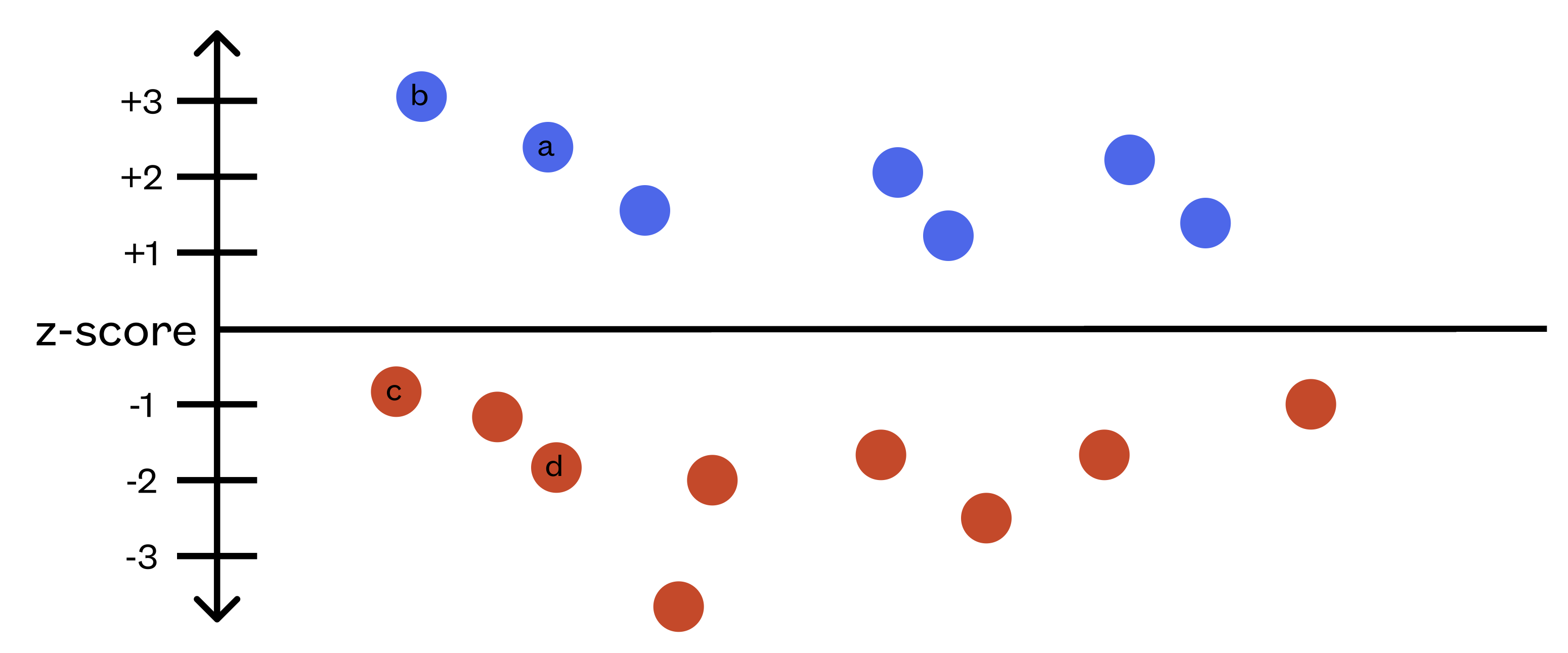
For instance, an equity with positive size exposure, such as equities a or b, is a Large-Cap equity while an equity with negative exposure, such as c or d, is a Small-cap equity. Since the exposures are computed on a normalized basis, we can easily compare the exposures among Large-cap equities as well: the one with higher (positive) size exposure, in this case b,  has a greater market capitalization than one with a smaller (positive) size exposure, in this case a.

We can now add the set of risk indices as extra factors to our factor model to complete the specification of the equity factor model:

To summarize, we have the following set of factors:

• Market Factor: Measures the dependence of any given equity's return on a global set of equities defined as the MSCI ACWI index.

• Country Factors: Measure the home country-specific dependence for individual equity. For equity ETFs or mutual funds, this set of factors measures the country-specific influences on the overall return of the ETF or mutual fund.

• Industry Factors: Similar to country factors, measure the industry-specific dependence for an individual equity, ETF, or mutual fund.

• Risk Indices: Measure the dependence of an individual equity's return on specific styles of investing or behavioral biases from investors. The exposures are computed on a relative basis against the baseline of the style-neutral MSCI ACWI Index.